
Skip to content

Grade 10 · Core Mathematics · Lesson 8 of 14

Drawing Velocity-Time Graphs from Data Tables: Deceleration and Scenarios

A Grade 10 Core Mathematics CBE lesson from the sub-strand Linear Motion. In it, learners plot velocity-time graphs from tabular data featuring non-zero initial velocities and uniform decelerations.

Strand Measurements and GeometrySub-strand Linear MotionLesson code 10CM-29-L840 minutes · 2 slides

KICD learning outcome (e)

Draw a velocity-time graph from given tables in different situations.

By the end of this lesson, learners should be able to

  1. Plot velocity-time graphs from tabular data featuring non-zero initial velocities and uniform decelerations.
  2. Construct velocity-time graphs accurately for practical multi-stage linear motion scenarios.

Key vocabulary

Deceleration
The reduction in an object's velocity per unit time, representing negative acceleration.
The boat has an acceleration of -15 km/h², i.e. a deceleration of 15 km/h².
Initial Velocity
The starting velocity of a moving object at time zero in a motion study.
The boat has an initial velocity of 75 km/h at t=0.
Multi-Stage Motion
Motion comprising several distinct phases with different accelerations or constant speeds over time.
The rocket exhibited multi-stage motion by accelerating then maintaining constant speed before landing.

Lesson preview

Slide 1 · Plotting Decreasing and Non-Zero Initial Velocity-Time GraphsModel · 18 min
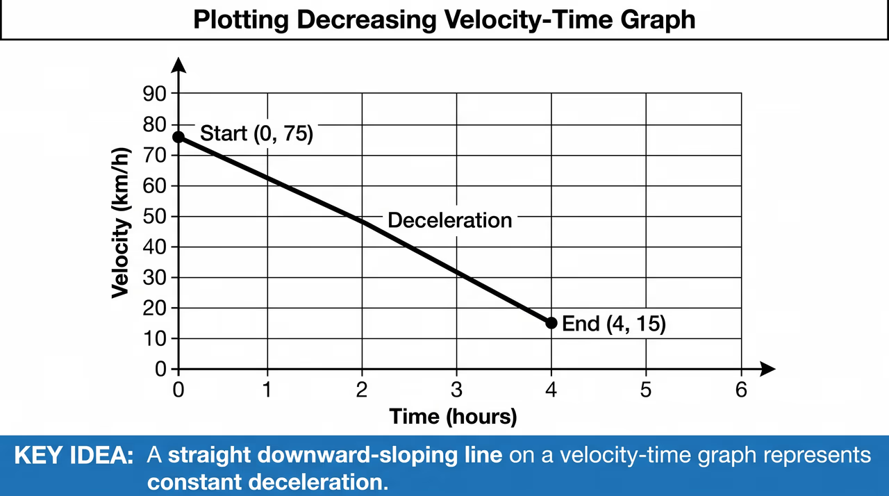
A velocity-time graph showing a straight downward-sloping line from a velocity of 75 km/h to 15 km/h over four hours, representing deceleration.
Figure 1: A velocity-time graph showing a straight downward-sloping line from a velocity of 75 km/h to 15 km/h over four hours, representing deceleration.

A velocity-time graph represents how velocity changes over time. When an object slows down or starts with an initial velocity, we choose consistent scale intervals for both axes. Time is plotted on the horizontal axis (x-axis) and velocity on the vertical axis (y-axis). Plotted points are joined using straight line segments. A downward slope indicates negative acceleration or deceleration, while a horizontal line indicates constant velocity. Use Figure 1 to see how a downward slope on a graph indicates deceleration.

  • Time is placed on the horizontal axis while velocity is placed on the vertical axis.
  • Always choose uniform, easy-to-read scale divisions for both graph axes before plotting coordinates.
  • Connect successive coordinate points with straight line segments using a straight edge or ruler.
  • A line sloping downwards from left to right indicates uniform deceleration or negative acceleration.
Worked example. Identify coordinate pairs (t,v) from the table: (0,75), (1,60), (2,45), (3,30), and (4,15). Draw the vertical axis for velocity in km/h marked from 0 up to 80 km/h and horizontal axis for time in hours marked from 0 to 5 h. Plot each point on graph paper using a sharp pencil and small crosses. Join the points with a ruler; read the y-intercept at t=0 h to find the initial velocity. Answer: Initial velocity is 75 km/h; the graph is a straight line sloping downwards from (0,75) to (4,15)..

Check question: An express bus decelerates uniformly. Its velocity, v, at time t is recorded as follows: at t=0 s, v=25 m/s; at t=2 s, v=20 m/s; at t=4 s, v=15 m/s. What is the y-intercept of the corresponding velocity-time graph?

  1. 0 m/s
  2. 15 m/s
  3. 20 m/s
  4. 25 m/s
Show answer

25 m/s. The y-intercept of a velocity-time graph represents the velocity when the time is t=0 s. From the data provided, at t=0 s, the velocity is 25 m/s. Therefore, the y-intercept is 25 m/s.

Slide 2 · Constructing Velocity-Time Graphs for Various Physical ScenariosPractice · 22 min
A velocity-time graph for a braking rally car, showing uniform deceleration as velocity decreases from 40 m/s to 0 m/s over four seconds.
Figure 2: A velocity-time graph for a braking rally car, showing uniform deceleration as velocity decreases from 40 m/s to 0 m/s over four seconds.

Teach the full lesson on the projector

This lesson, and every other Grade 1–10 CBE lesson, comes ready to project with the EAP ClassKit. It runs without electricity or internet.

  • Both slides with diagrams and class activities
  • Teacher notes, SNE adaptations and assessment checks
  • Homework and the other 13 lessons in this sub-strand

All 14 lessons in Linear Motion

  1. 1Distance, Displacement, Speed, Velocity and AccelerationExplain the terms distance, displacement, speed, velocity and acceleration in real-life situations
  2. 2Determining Velocity and AccelerationDetermine velocity and acceleration in different situations
  3. 3Determining Velocity and Acceleration in Different SituationsDetermine velocity and acceleration in different situations
  4. 4Drawing Displacement-Time Graphs in Linear MotionDraw a displacement-time graph of different situations
  5. 5Interpreting Displacement-Time GraphsInterpret displacement-time graph in different situations
  6. 6Interpreting Displacement-Time Graphs in Different SituationsInterpret displacement-time graph in different situations
  7. 7Drawing Velocity-Time Graphs from Data TablesDraw a velocity-time graph from given tables in different situations
  8. 8Drawing Velocity-Time Graphs from Data Tables: Deceleration and ScenariosDraw a velocity-time graph from given tables in different situations
  9. 9Interpreting Velocity-Time Graphs in Linear MotionInterpret velocity-time graph in different situations
  10. 10Interpreting Velocity-Time Graphs in Practical SituationsInterpret velocity-time graph in different situations
  11. 11Relative Speed in Linear MotionDetermine relative speed of two moving bodies in different situations
  12. 12Relative Speed in Linear Motion: Advanced ApplicationsDetermine relative speed of two moving bodies in different situations
  13. 13Appreciating Linear Motion in Real-Life SituationsAppreciate use of linear motion in real-life situations
  14. 14Real-Life Applications of Linear MotionAppreciate use of linear motion in real-life situations