Drawing Displacement-Time Graphs in Linear Motion

By the end of this lesson, learners should be able to

1. Select appropriate axis scales and construct a displacement-time graph from a given table of values.
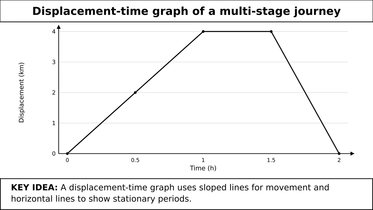
2. Draw a multi-stage displacement-time graph representing real-life journey scenarios with rest periods and return trips.

Key vocabulary

Displacement-time graph

A graph showing an object's position relative to a reference point plotted against elapsed time.

The displacement-time graph shows the van reached $8\text{ km}$ from the warehouse after $20\text{ minutes}$.

Scale factor

The ratio between a length represented on graph grid lines and the actual quantity measured.

Choosing a scale factor of $1\text{ cm}$ to $5\text{ minutes}$ makes plotting tabular times effortless.

Cumulative elapsed time

The total time passed since the beginning of a multi-stage journey or motion event.

From 9:00 am to 9:30 am, the cumulative elapsed time is 30 minutes.

Stationary stage

A time interval during linear motion where an object remains at a fixed position.

Waiting at a bus stop for 20 minutes forms a horizontal stationary stage on the graph.

Lesson preview

Slide 1 · Constructing Displacement-Time Graphs from Tabular DataModel · 18 min

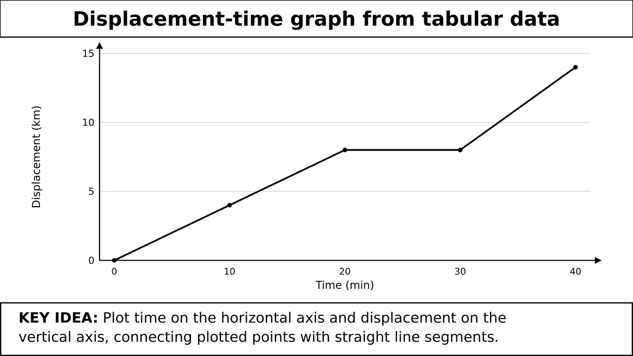
A displacement-time graph shows how an object's position changes relative to a starting reference point over time. Time is placed on the horizontal axis and displacement on the vertical axis. We choose clear, uniform scales so all data points fit neatly. By plotting recorded coordinate pairs $(t,s)$ from a data table and connecting successive points with straight lines, we construct a continuous line graph that visualises linear motion. Use Figure 1 to see how connecting recorded coordinate pairs works.

• Plot time along the horizontal axis and displacement along the vertical axis using uniform axis scales.
• Choose scale factors that cover the full range of data conveniently on grid paper.
• Mark coordinate points accurately from the recorded table of times and displacements.
• Connect adjacent plotted coordinates using straight line segments to complete the displacement-time graph.

Worked example. Identify ranges: time $t$ ranges from $0$ to $40\text{ min}$ ($40\text{ min}$ span), displacement $s$ ranges from $0$ to $14\text{ km}$ ($14\text{ km}$ span). Choose horizontal scale: Let $1\text{ cm}$ represent $5\text{ min}$, taking $8\text{ cm}$ along the horizontal $t$-axis. Choose vertical scale: Let $1\text{ cm}$ represent $2\text{ km}$, taking $7\text{ cm}$ along the vertical $s$-axis. Plot the coordinates $(0,0)$, $(10,4)$, $(20,8)$, $(30,8)$, and $(40,14)$, then join consecutive points with straight line segments. Answer: Horizontal scale: $1\text{ cm}=5\text{ min}$; Vertical scale: $1\text{ cm}=2\text{ km}$. Points $(0,0)$, $(10,4)$, $(20,8)$, $(30,8)$, $(40,14)$ joined sequentially..

Check question: A runner's displacement from a starting line reaches a maximum of $300\text{ m}$ over $15\text{ minutes}$. Which vertical scale will make the $300\text{ m}$ peak fit exactly into a $6\text{ cm}$ vertical grid height?

1. $1\text{ cm}=20\text{ m}$
2. $1\text{ cm}=50\text{ m}$
3. $1\text{ cm}=60\text{ m}$
4. $1\text{ cm}=100\text{ m}$

Show answer

$1\text{ cm}=50\text{ m}$. To find the correct scale, divide the maximum displacement by the available grid height: $300\text{ m}÷6\text{ cm}=50\text{ m/cm}$. Therefore, the scale $1\text{ cm}=50\text{ m}$ uses exactly $6\text{ cm}$ of the grid.

Slide 2 · Plotting Multi-Stage Journeys and Narrative Motion ScenariosPractice · 22 min

Teach the full lesson on the projector

This lesson, and every other Grade 1–10 CBE lesson, comes ready to project with the EAP ClassKit. It runs without electricity or internet.

• Both slides with diagrams and class activities
• Teacher notes, SNE adaptations and assessment checks
• Homework and the other 13 lessons in this sub-strand

See the school projectorWhatsApp us

All 14 lessons in Linear Motion

1. 1Distance, Displacement, Speed, Velocity and AccelerationExplain the terms distance, displacement, speed, velocity and acceleration in real-life situations
2. 2Determining Velocity and AccelerationDetermine velocity and acceleration in different situations
3. 3Determining Velocity and Acceleration in Different SituationsDetermine velocity and acceleration in different situations
4. 4Drawing Displacement-Time Graphs in Linear MotionDraw a displacement-time graph of different situations
5. 5Interpreting Displacement-Time GraphsInterpret displacement-time graph in different situations
6. 6Interpreting Displacement-Time Graphs in Different SituationsInterpret displacement-time graph in different situations
7. 7Drawing Velocity-Time Graphs from Data TablesDraw a velocity-time graph from given tables in different situations
8. 8Drawing Velocity-Time Graphs from Data Tables: Deceleration and ScenariosDraw a velocity-time graph from given tables in different situations
9. 9Interpreting Velocity-Time Graphs in Linear MotionInterpret velocity-time graph in different situations
10. 10Interpreting Velocity-Time Graphs in Practical SituationsInterpret velocity-time graph in different situations
11. 11Relative Speed in Linear MotionDetermine relative speed of two moving bodies in different situations
12. 12Relative Speed in Linear Motion: Advanced ApplicationsDetermine relative speed of two moving bodies in different situations
13. 13Appreciating Linear Motion in Real-Life SituationsAppreciate use of linear motion in real-life situations
14. 14Real-Life Applications of Linear MotionAppreciate use of linear motion in real-life situations